How to build a Recommender System in TensorFlow
Introduction
First of all, I’ll start with a definition. A recommender system is a software that exploits user’s preferences to suggests items (movies, products, songs, events, etc…) to users. It helps users to find what they are looking for and it allows users to discover new interesting never seen items.
Deep Learning is acquiring great notoriety nowadays because of the leverage of substantial computational power and its capacity to solve complex tasks such as image recognition, natural language processing, speech recognition, and so on.
It has proven to be useful also in the recommendation problem which consists in predicting an estimation function of how much a user $u$ will be interested in item $i$ for unseen items.
\[R : Users \times Items \rightarrow Ratings\]Two different approaches may be adopted to solve the recommendation problem:
- Content-Based
- Collaborative Filtering
The former exploits items’ description to infer a rate, the latter exploits users’ neighborhood, so it’s based on the concept that similar users give similar rate to items. In this post, we will cover the Collaborative Filtering approach.
Tutorial
In this tutorial we are going to build a recommender system using TensorFlow. We’ll use other useful packages such as:
- NumPy: scientific computing in Python;
- Pandas: data analysis library, very useful for data manipulation.
Let’s import all of them!
import numpy as np
import pandas as pd
import tensorflow as tf
Download the MovieLens 1M dataset which contains 1 million ratings from 6000 users on 4000 movies. Ratings are contained in the file “ratings.dat” in the following format:
UserID::MovieID::Rating::Timestamp
You can convert easily ratings file in a TSV (Tab-Separated Values) file with the following bash command:
$ sed -i -e 's/::/\t/g' ratings.datWe have to split our dataset in a training set and a test set. The training set is used to train our model, and the test set will be used only to evaluate the learned model. We split the dataset using the Hold-Out 80/20 protocol, so 80% of ratings for each user are kept in the training set, the remaining 20% will be moved to the test set. If you have a dataset with few ratings, the best choice for splitting protocol would be the K-Fold.
Let’s load the dataset with pandas:
# Reading dataset

df = pd.read_csv('train-1m.tsv', sep='\t', names=['user', 'item', 'rating', 'timestamp'], header=None)
df = df.drop('timestamp', axis=1)

num_items = df.item.nunique()
num_users = df.user.nunique()

print("USERS: {} ITEMS: {}".format(num_users, num_items))
Pandas will load training set into a DataFrame with three columns: user, item and ratings.
# Normalize in [0, 1]

r = df['rating'].values.astype(float)
min_max_scaler = preprocessing.MinMaxScaler()
x_scaled = min_max_scaler.fit_transform(r.reshape(-1,1))
df_normalized = pd.DataFrame(x_scaled)
df['rating'] = df_normalized
Pandas DataFrames cannot be directly used to feed a model, the best option is to convert a DataFrame into a matrix:
# Convert DataFrame in user-item matrix

matrix = df.pivot(index='user', columns='item', values='rating')
matrix.fillna(0, inplace=True)
Rows in the matrix correspond to users and columns to items; therefore entries correspond to ratings given by users to items. Our matrix is still an object of DataFrame type, we need to convert it to a numpy matrix.
# Users and items ordered as they are in matrix

users = matrix.index.tolist()
items = matrix.columns.tolist()

matrix = matrix.as_matrix()
Finally, we can start to set up some network parameters, such as the dimension of each hidden layer, in this tutorial we will use 2 hidden layers.
X is a placeholder, it just tells to TensorFlow that we have a variable X in the computational graph.
Weights and biases are dictionaries of variables, randomly initialized of type float.
# Network Parameters

num_input = num_items
num_hidden_1 = 10
num_hidden_2 = 5

X = tf.placeholder(tf.float64, [None, num_input])

weights = {
    'encoder_h1': tf.Variable(tf.random_normal([num_input, num_hidden_1], dtype=tf.float64)),
    'encoder_h2': tf.Variable(tf.random_normal([num_hidden_1, num_hidden_2], dtype=tf.float64)),
    'decoder_h1': tf.Variable(tf.random_normal([num_hidden_2, num_hidden_1], dtype=tf.float64)),
    'decoder_h2': tf.Variable(tf.random_normal([num_hidden_1, num_input], dtype=tf.float64)),
}

biases = {
    'encoder_b1': tf.Variable(tf.random_normal([num_hidden_1], dtype=tf.float64)),
    'encoder_b2': tf.Variable(tf.random_normal([num_hidden_2], dtype=tf.float64)),
    'decoder_b1': tf.Variable(tf.random_normal([num_hidden_1], dtype=tf.float64)),
    'decoder_b2': tf.Variable(tf.random_normal([num_input], dtype=tf.float64)),
}
Let’s now define our model. Autoencoders are unsupervised learning neural networks, they try to reconstruct input data at the output, this means that they learn a compressed representation of the input, and they use that to reconstruct the output.
# Building the encoder

def encoder(x):
    # Encoder Hidden layer with sigmoid activation #1
    layer_1 = tf.nn.sigmoid(tf.add(tf.matmul(x, weights['encoder_h1']), biases['encoder_b1']))
    # Encoder Hidden layer with sigmoid activation #2
    layer_2 = tf.nn.sigmoid(tf.add(tf.matmul(layer_1, weights['encoder_h2']), biases['encoder_b2']))
    return layer_2


# Building the decoder

def decoder(x):
    # Decoder Hidden layer with sigmoid activation #1
    layer_1 = tf.nn.sigmoid(tf.add(tf.matmul(x, weights['decoder_h1']), biases['decoder_b1']))
    # Decoder Hidden layer with sigmoid activation #2
    layer_2 = tf.nn.sigmoid(tf.add(tf.matmul(layer_1, weights['decoder_h2']), biases['decoder_b2']))
    return layer_2


# Construct model

encoder_op = encoder(X)
decoder_op = decoder(encoder_op)


# Prediction

y_pred = decoder_op


# Targets are the input data.

y_true = X
Once the structure of a neural network has been defined, we need a loss function. A loss function quantifies how much worse is our estimate on the current example, using the current parameters W for the model. The cost function is just the average of the loss function over all the samples in the training set. Said that we want to minimize our loss. A different optimizer can be used such as Adam, Adagrad, Adadelta, and others.
# Define loss and optimizer, minimize the squared error

loss = tf.losses.mean_squared_error(y_true, y_pred)
optimizer = tf.train.RMSPropOptimizer(0.03).minimize(loss)

predictions = pd.DataFrame()

# Define evaluation metrics

eval_x = tf.placeholder(tf.int32, )
eval_y = tf.placeholder(tf.int32, )
pre, pre_op = tf.metrics.precision(labels=eval_x, predictions=eval_y)
Because of TensorFlow uses computational graphs for his operations, placeholders and variables must be initialized, at this point, no more variables can be allocated.
# Initialize the variables (i.e. assign their default value)

init = tf.global_variables_initializer()
local_init = tf.local_variables_initializer()
We can finally start to train our model.
We split training data into batches, and we feed the network with them. Using mini-batch technique is useful to speed up the training because weights are updated one time per batch. You may also think to shuffle your mini-batches to make the gradient more variable; hence it can help to converge because it increases the likelihood of hitting a good direction and prevents some local minima.
We train our model with vectors of user ratings, each vector represents a user and each column an item. As previously said, entries are ratings that the user gave to items. The main idea is to encode input data in a smaller space, a meaningful representation for users based on their rating, to predict unrated items.
Let’s back to the code, we are going to train our model for 100 epochs with a batch size of 250. This means that the entire training set will feed our neural network 100 times, every time using 250 users.
At the end of training, the encoder will contain a compact representation of the input data. We will then use the decoder to reconstruct the original user rating, but this time we will have a score even for unrated user’s items based on the learned representation for other users.
with tf.Session() as session:
    epochs = 100
    batch_size = 250

    session.run(init)
    session.run(local_init)

    num_batches = int(matrix.shape[0] / batch_size)
    matrix = np.array_split(matrix, num_batches)

    for i in range(epochs):

        avg_cost = 0

        for batch in matrix:
            _, l = session.run([optimizer, loss], feed_dict={X: batch})
            avg_cost += l

        avg_cost /= num_batches

        print("Epoch: {} Loss: {}".format(i + 1, avg_cost))

    print("Predictions...")

    matrix = np.concatenate(matrix, axis=0)

    preds = session.run(decoder_op, feed_dict={X: matrix})

    predictions = predictions.append(pd.DataFrame(preds))

    predictions = predictions.stack().reset_index(name='rating')
    predictions.columns = ['user', 'item', 'rating']
    predictions['user'] = predictions['user'].map(lambda value: users[value])
    predictions['item'] = predictions['item'].map(lambda value: items[value])
We are ready to evaluate our model, but first, user’s ratings in the training set must be removed. We keep only the top-10 ranked items for each user.
    print("Filtering out items in training set")

    keys = ['user', 'item']
    i1 = predictions.set_index(keys).index
    i2 = df.set_index(keys).index

    recs = predictions[~i1.isin(i2)]
    recs = recs.sort_values(['user', 'rating'], ascending=[True, False])
    recs = recs.groupby('user').head(10)
    recs.to_csv('recs.tsv', sep='\t', index=False, header=False)
Evaluation
How do we evaluate a recommender system?
A good predictor is not always a good recommender, that’s why all prediction metrics should be avoided instead of ranking metrics from Information Retrieval field.
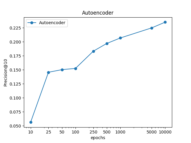
In this tutorial, we will use the Precision@10 metric, which evaluates (for each user) if an item in the predicted top-10 is contained in the top-10 items in the test set.
Formally it is defined as:
\[Precision@N = \frac{|L_{u}(N) \cap TS_{u}^{+}|}{N}\]where $L_{u}(N)$ is the recommendation list up to the N-th element and $TS_{u}^{+}$ is the set of relevant test items for $u$. Precision measures the system’s ability to reject any non-relevant documents in the retrieved set.
In the following plot, we can see how much increase in precision we can obtain with more epochs. Be aware that training with many epochs beyond necessary would not be the best option because you may fit great training data, but you may lose generalization capacity on the test set. To find the optimal number of epochs you have to use a validation set and check for each epoch the loss on that set. When loss on validation set begins to increase, you can stop the training at that epoch.
To evaluate the recommendation I suggest to use an open source library called RankSys, written in Java, it’s really fast, and it implements many ranking metrics.
Conclusion
You are now able to build a recommender system with the same performances of other Collaborative Filtering algorithms such as Matrix Factorization.
You can play with network settings such as hidden layers’ dimension as see how system’s performances change. Generally, their dimension depends on the complexity of the function you want to approximate. If your hidden layers are too big, you may experience overfitting and your model will lose the capacity to generalize well on the test set. On the contrary, if they are too small, the neural network would not have enough parameters to fit well the data. You may also want to improve performances trying some regularization techniques like the dropout.
Code
Code available at tfautorec.